Learning Rust by Simulating Heat Diffusion
In the summer of 2018, Rust caught my attention. For most people, C++ is the
primary choice for any job that requires fast performance. Even though I also
dabbled in some front-end tech like React and the whole tangled mess of NPM
Dependency Hell™
(cough leftpad),
I thought it was strange that C++, the language that is most people’s first
choice for writing fast, low-level code, feels like 30 years of afterthoughts
carefully glued onto each other. We have learned many things about programming
in 30 years.
This is what made me so excited to find Rust, a language that is not only fun to
code in and (after the initial learning curve) highly intuitive, but also
lightning-fast and with opinionated tools. It combines the delight of
npm installing some random package dumped into the package registry and
watching your program execute in a fraction of a second, thanks to the package
manager cargo and an LLVM-backed compiler. I could now pull in other people’s
polluted, bloated code and obsess over shaving off microseconds of execution
at the same time. Unsurprisingly, I like math and physics. While learning Rust,
it happened that I was curious about implementing a numerical method for the
heat equation, which is a partial differential equation (PDE) that models heat
diffusion in most materials:
$$ \frac{\partial u}{\partial t} = - a \nabla^2 u $$
This equation says that the rate of change of heat ($\frac{\partial u}{\partial t}$) is proportional to the Laplacian of the heat distribution ($ \nabla^2 u$) at that point. The Laplacian operator tells you how different a point is compared to its neighbors. If the point is, on average, less than its neighbors, the Laplacian will be positive, and vice versa. This equation captures your intuition that a spot much hotter or colder than its neighbors will equalize faster.
I chose to simulate heat diffusion because it’s relatively simple compared to other analytic systems, like waves or fluid.
Math
Since we’re concerned with running a simulation, we have to use discrete steps in time and space instead of an infinitely detailed continuum, assigning a certain heat value to every point and determining what it will be at the next moment. What’s so great about the heat equation is that, for each point, I can compute the first time derivative in terms of its current state in position space. Since I know how fast each point is changing, I can model the time evolution of the system! Although I wanted to eventually create a higher dimension simulation, I had to start in 1D.
Recalling the original heat equation, the change in heat $du$ is proportional to the Laplacian times the infinitesimal time step $dt$. However, we have to convert each differential operator into a discrete equivalent. The discrete Laplacian is actually quite simple in one dimension. You simply add the neighbors and subtract two times the point to evaluate the lowest order approximation of the Laplacian at that point. The finite difference equation
$$ \frac{u^{n+1}_j-u^n_j}{k} = \frac{u^n_{j+1} - 2u^n_j + u^n_{j-1}}{h^2} $$
models our heat distribution $u$, where the subscript is the space index and superscript is the time index. This formula, shamelessly ripped from Wikipedia, replaces the derivatives in the heat equation with finite difference approximations. A derivative is defined as the slope of a tangent line, which in turn is the limit of secant lines through the function at a target point and another point arbitrarily close. The finite difference simply picks another point so that one can approximate the derivative. (To get the approximation of the Laplacian on the right-hand side, use the definition of the derivative twice, but replace the arbitrarily small step with a finite one.)

The limit of secant lines is a tangent line. Since derivatives are slopes of tangent lines, they can be approximated by slopes of secant lines using a finite difference quotient.
In the finite difference approximation, the $k$ corresponds to $dt$, or the time step we will use. $h$ corresponds to the position step. Wikipedia notes that the numerical method is stable for $r=\frac{k}{h^2} \leq 0.5$. Otherwise, each iteration of our simulation will gradually lead to more extreme and useless values.
Gallery
I produced these images with my final version of the heat simulation program,
which includes another variant that works on 2D space. These are plotted with
the library gnuplot.
These are simulations of heat distribution along one or two spatial dimensions, starting with a single spike, or impulse, of heat at the center and letting it diffuse. It’s no accident that these look like normal distributions' bell curves — the impulse response/Green’s function of the heat PDE, is actually a normal distribution that spreads out over time.
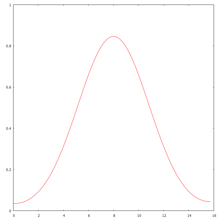
1D heat @ 16 initial spike, 4 time units, 64 position bins, 16 position units wide. This is the plot that corresponds to the abridged program above.
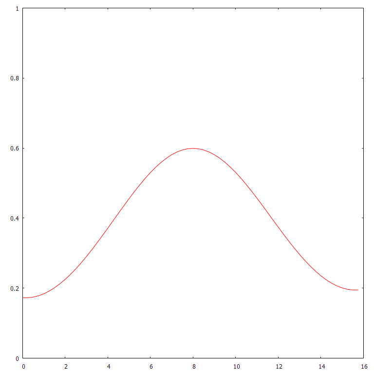
1D heat @ 16 initial spike, 8 time units, 64 position bins, 16 position units wide.
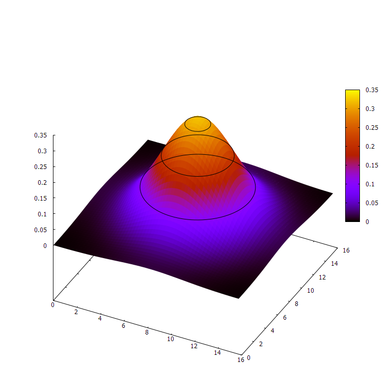
2D heat @ 16 initial spike, 4 time units, 64² position bins, 64 position units wide. Note the z-scale.
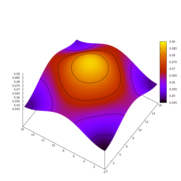
2D heat @ 16 initial spike, 16 time units, 64² position bins, 64 position units wide. Note the z-scale.
Code
We’ll walk through creating a 1D heat simulation and plotting it. This isn’t exactly how I did it — which involved a lot of trial and error — but it’s pretty close.
Writing the simulation
Let’s create a file called heat.rs to contain our simulation’s heavy lifting.
We will run the simulation with a separate file.
First, we create a struct Heat1D to encapsulate the data and functionality of
a one dimensional heat simulation. The pub keyword exposes the struct and its
fields outside the module. This type of struct is known as a tuple struct, since
it is essentially a named tuple type. The single element in the tuple is a
vector of 64-bit floats (doubles), Vec<f64>. It contains the state of the
simulation at a given time. The function step in the impl block will compute
a time step given the $r$ value from above. step also mutably borrows the
Heat1D object it is called on, allowing it to change the values in the
Vec<f64>.
In heat.rs:
| |
Every time we call the step method, we want the system to advance in time
according to the $r$ value. Our Laplacian isn’t defined for points without
neighbors, so the method should not change the edges. To compute the Laplacian,
we need to iterate over each value in the vector, making a copy of the previous
value and peeking at the next value. Instead of doing this by incrementing an
index (boring!), we can use Rust’s iterators.
In the body of step:
| |
On line 2, we use .0 to access the enclosed Vec<f64>, get an iterator that
allows you to change elements, and allow peeking of the next value. Line 4 uses
the special syntax if let, which attempts to match the value on the right to
the pattern on the left. Some, along with None, are the enum variants of
Option, which acts as an optional value — think Java’s nullable pointers
or C++’s std::optional. Similarly, the while let loop on line 4 terminates
when there is no longer an element after the current one.
Next, we need to update cur while copying it to prev for use in the
following computation. We could just make a copy of the whole vector, but
where’s the fun in that? prev is a plain f64, so it needs no dereferencing.
cur is a mutable reference to an f64 (&mut f64), which allows us to change
it, but it needs one use of the dereference operator * to access its data.
Since we peek next, it’s actually a &&mut f64, so we need to dereference it
twice!
| |
The type f64 implements a special Rust trait called Copy, which indicates
that any assignments will copy the data instead of moving it and rendering the
initial value useless. All Rust primitives are Copy. However, structs and
enums are not Copy by default. To finish our simulation, we will add a method
called copy_edges. This method will copy the heat values next to each edge to
the edge itself. If we call copy_edges before every time step, then heat will
neither escape nor enter via the edges, since the neighboring cells have the
same heat value, simulating a closed system.
| |
Running the simulation
Now, we can create a main.rs file to actually run the simulation. We use mod
to declare the existence of heat.rs so we can access its contents. Then, we
utilize the use keyword to bring our Heat1D struct into the scope so we
don’t have to type its fully qualified name all the time.
In main.rs:
| |
We need a few parameters for our simulation, namely the physical size of the
simulation, duration we will simulate, and the resolution of space and time our
program will use. We can then use these parameters to compute $r$, the ratio
between our discrete Laplacian and the change in heat at each point. We’ll make
SIM_SIZE the number of space bins we will split our one-dimensional interval
in. Rust requires that we declare the type of compile-time constants. We use
type usize because it represents a count, which in this case, is 64 evenly
spaced points in space.
| |
Then, we define the width of the of the simulation as 16 “unit lengths.” Note
that we use the type f64, or a 64-bit float. This is a double in other
languages.
| |
We do a similar thing for the time scale, using 2048 steps and running the simulation for 8 “unit durations.”
| |
Now we create our main function. Rust will call this function in the main file
when the program is run as a binary. We compute $h$, $k$, and $r$, and use the
assert! macro to ensure that $r \leq 0.5$. If it isn’t, the simulation is
unstable and will fail to converge. The assert! terminates the program if this
condition is false, guaranteeing that the simulation is stable.
| |
We must cast the usizes to f64s using the as keyword, since Rust
purposefully avoids implicit casting in exchange for compiler type inference. In
our main method, we create a Heat1D instance, utilizing the vec! macro to
make SIM_SIZE number of bins, all set to 0. In the center, we set an initial
spike of heat of arbitrary magnitude to let diffuse. This represents the initial
conditions for our simulation.
| |
We can use the println! macro to print the contents of the simulation. The
{:?} syntax formats any object that implements the Debug trait, such as our
Vec of floats.
| |
We run the simulation’s step function for as many steps as SIM_STEPS,
copying the edges each time to simulate a closed system. This for loop
iterates over a range, using the _ syntax is used to discard the iteration
variable.
| |
After the simulation is done, we print the final array.
| |
When run, this should give us something like
| |
which is impressive! The final heat distribution seems to increase towards the
center, but unfortunately a list of numbers is a pain to read. I took the time
to install the gnuplot crate using
cargo and the native library it hooks into so that
I could plot the data. I added this code at the end of main to generate the
images below.
| |
And we’re done!
Abridged Source
The complete program can be found at this gist.
heat.rs
| |
main.rs
| |
Conclusion
This project was pretty fun. It turns out that simulating such a simple system as heat diffusion is relatively easy. The Rust borrow checker helped keep my code bug-free and kept me focused on the logic of my program rather than the technical details. Also, the graphs look really cool, which is of course the most important part.